Introduction

To assess how general the measurements of SpatIS and SpatICS are for different contexts and populations, here we simulate populations in which individuals vary both in their most visited places and in their fidelity to those places. Doing that allows us to simulate both specialist and generalist populations, as well as vary the degree of individual specialization within the populations.

For the sake of simplicity, we assume that individual utilization distributions (UDs) are one dimensional (UD(x) instead of UD(x,y)) and follow a Gaussian distribution. The mean of the UD represents the location (in x) of the most visited place for a given individual, while the standard deviation (SD) of the UD represents their site fidelity (low SD indicates high site fidelity).

Here we create four scenarios and calculate the individual and population SpatIS and SpatICS for them. The scenarios are: (i) specialist individuals with different UD means and low between-individual variation in UD width, (ii) generalist individuals with similar UD means and low variation in UD width, (iii) specialist individuals with different UD means and with high variation in UD width, and (iv) specialist individuals with similar UD means but high variation in UD width.

1 The typical specialist population: specialist individuals with different UD means and low variation in UD width

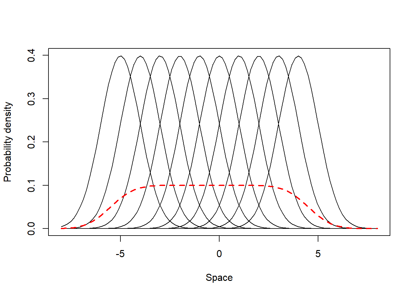
This scenario comprises individuals which are specialists in their most visited places (i.e. have different mean UD values) but do not present individual variation in their site fidelity - all individuals have UDs with similar SD, which are small compared to the populational UD standard deviation. Below we simulate and illustrate such a population. In this and all the examples along this appendix, the black lines represent the UD of the individuals and the red line the population UD.

# Specialist individuals, no SD variation

# simulate 10 individuals

# individual UD mean
avg.specialist.low <- seq(-5, 4, 1)
# individual UD SD
sd.specialist.low <- 1

# Populational UD
pop.curve <- function(x, mn, sd) {
  f <- 0
  for(i in mn) f <- f + dnorm(x, mean = i, sd = sd)
  f/length(mn)
}
# Making sure it integrates to 1
integrate(pop.curve, lower = -Inf, upper = Inf, mn = avg.specialist.low, 
          sd = sd.specialist.low)

## 1 with absolute error < 4.7e-06

# Plot
plot(0, 0, type = "n", xlim = c(-8,8), ylim = c(0, .4),
     xlab = "Space", ylab = "Probability density")
for(i in avg.specialist.low) curve(dnorm(x, mean = i, sd = sd.specialist.low), 
                                   from = -8, to = 8, add = T)
curve(pop.curve(x, mn = avg.specialist.low, sd = sd.specialist.low),
      from = -8, to = 8, lwd = 2, lty = 2, col = 2, add = T)

Now we calculate SpatIS and SpatICS using the equation presented in the main text of Kerches-Rogeri et al. Both the populational (SpatIS = 0.62, SpatICS = 0.69) and individual values are relatively high (SpatIS in the range [0.57, 0.73], SpatICS in the range [0.63, 0.82]), as expected. This indicates a specialist population composed of specialist individuals.

# declare SpatIS function 
spatis <- function(i) {
  1 - integrate(function(x, md) 
    pmin(dnorm(x, mean = md, sd = sd.specialist.low), 
         pop.curve(x, mn = avg.specialist.low, sd = sd.specialist.low)), 
    lower = -Inf, upper = Inf, md = i)$value
}
  
# declare SpatICS function
spatics <- function(i) {
  1 - integrate(function(x, md) 
    pmin(dnorm(x, mean = md, sd = sd.specialist.low), 
         pop.curve(x, mn = avg.specialist.low[avg.specialist.low != md], sd = sd.specialist.low)), 
    lower = -Inf, upper = Inf, md = i)$value 
}

# calculate SpatIS
# individual values
sapply(avg.specialist.low, spatis)

##  [1] 0.7351490 0.6368802 0.5826019 0.5721302 0.5711332 0.5711303 0.5721286
##  [8] 0.5826039 0.6368784 0.7351494

# populational value
mean(sapply(avg.specialist.low, spatis))

## [1] 0.6195785

# calculate SpatICS
# individual values
sapply(avg.specialist.low, spatics)

##  [1] 0.8168322 0.7076447 0.6473354 0.6357002 0.6345924 0.6345893 0.6356981
##  [8] 0.6473377 0.7076429 0.8168326

# populational value
mean(sapply(avg.specialist.low, spatics))

## [1] 0.6884206

2 The typical generalist population: generalist individuals with similar UD means and low variation in UD width

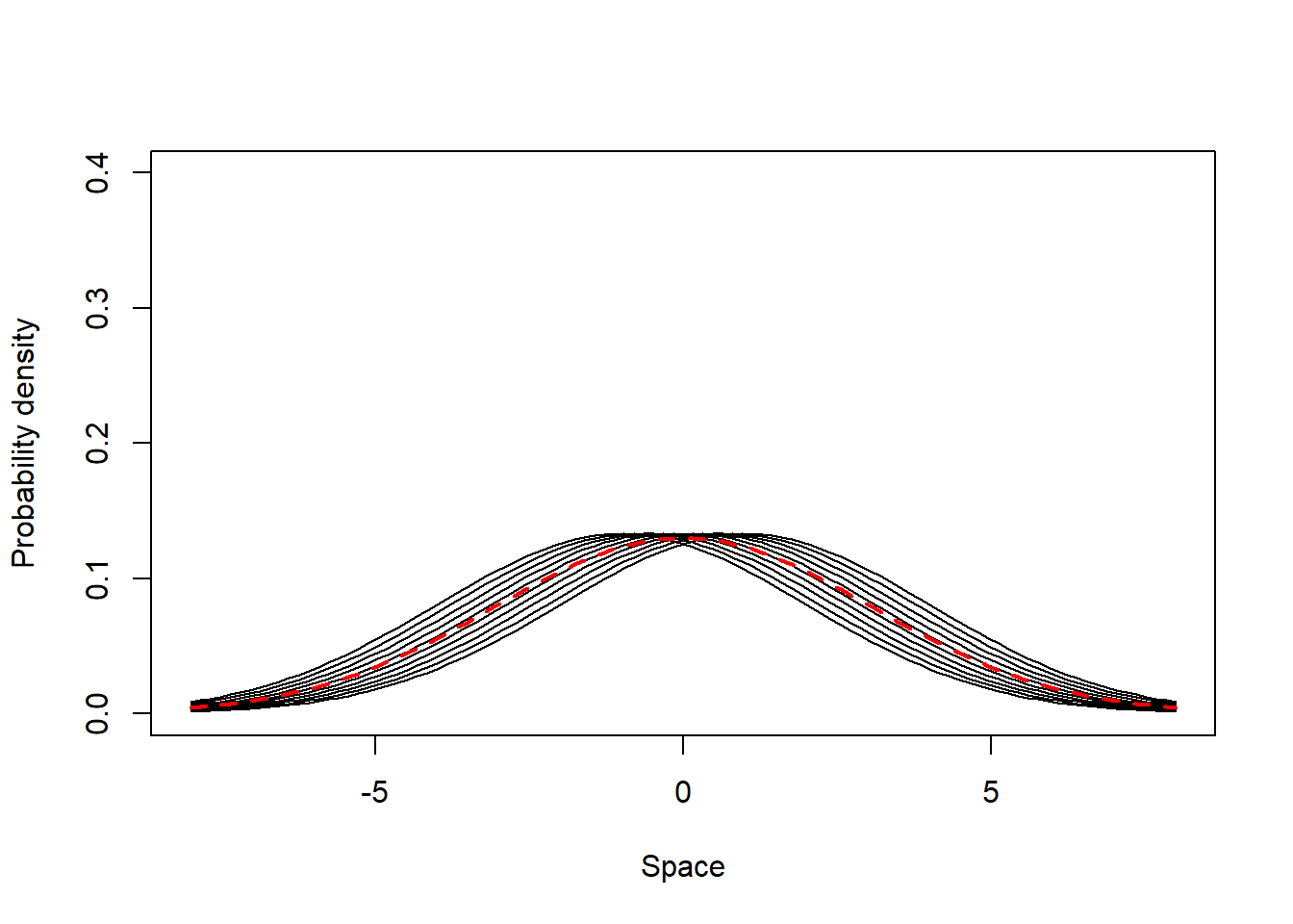
This scenario comprises individuals which are generalist in their most visited places (i.e. have mean UD values close to each other) and present very low site fidelity. All individuals have UDs with similar SD, which is large compared to the populational UD standard deviation. Below we simulate and illustrate such a population.

# Generalist individuals, no SD variation

# simulate 10 individuals

# individual UD mean
avg.specialist.low <- seq(-1, 1, length.out = 10)
# individual UD SD
sd.specialist.low <- 3

# Populational UD
pop.curve <- function(x, mn, sd) {
  f <- 0
  for(i in mn) f <- f + dnorm(x, mean = i, sd = sd)
  f/length(mn)
}
# Making sure it integrates to 1
integrate(pop.curve, lower = -Inf, upper = Inf, mn = avg.specialist.low, 
          sd = sd.specialist.low)

## 1 with absolute error < 3.3e-07

# Plot
plot(0, 0, type = "n", xlim = c(-8,8), ylim = c(0, 0.4),
     xlab = "Space", ylab = "Probability density")
for(i in avg.specialist.low) curve(dnorm(x, mean = i, sd = sd.specialist.low), 
                                   from = -8, to = 8, add = T)
curve(pop.curve(x, mn = avg.specialist.low, sd = sd.specialist.low), 
      from = -8, to = 8, lwd = 2, lty = 2, col = 2, add = T)

Both the populational (SpatIS = 0.07, SpatICS = 0.08) and individual values are low (SpatIS in the range [0.017, 0.13], SpatICS in the range [0.019, 0.146]), as expected. This indicates a generalist population composed of generalist individuals.

# declare SpatIS function 
spatis <- function(i) {
  1 - integrate(function(x, md) 
    pmin(dnorm(x, mean = md, sd = sd.specialist.low), 
         pop.curve(x, mn = avg.specialist.low, sd = sd.specialist.low)), 
    lower = -Inf, upper = Inf, md = i)$value
}
  
# declare SpatICS function
spatics <- function(i) {
  1 - integrate(function(x, md) 
    pmin(dnorm(x, mean = md, sd = sd.specialist.low), 
         pop.curve(x, mn = avg.specialist.low[avg.specialist.low != md], 
                   sd = sd.specialist.low)), 
    lower = -Inf, upper = Inf, md = i)$value 
}

# calculate SpatIS
# individual values
sapply(avg.specialist.low, spatis)

##  [1] 0.13119577 0.10237683 0.07348818 0.04469291 0.01726530 0.01726530
##  [7] 0.04469291 0.07348818 0.10237683 0.13119577

# populational value
mean(sapply(avg.specialist.low, spatis))

## [1] 0.0738038

# calculate SpatICS
# individual values
sapply(avg.specialist.low, spatics)

##  [1] 0.14577308 0.11375203 0.08165353 0.04965879 0.01918414 0.01918414
##  [7] 0.04965879 0.08165353 0.11375203 0.14577308

# populational value
mean(sapply(avg.specialist.low, spatics))

## [1] 0.08200431

3 In-between: individuals with different UD means and a varying degree of site fidelity

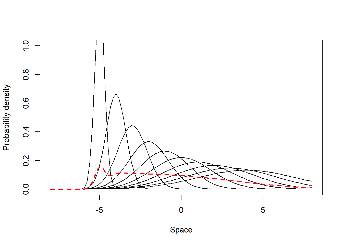
This scenario comprises individuals which are specialists in their most visited places (i.e. have different mean UD values) but present a gradient of individual variation in their site fidelity - some individuals have UDs with small SD (high site fidelity), while others have UDs with high SD compared to the populational UD standard deviation (low side fidelity). Below we simulate and illustrate such a population.

# Specialist individuals, high interindividual SD variation

# simulate 10 individuals

# individual UD mean
avg.specialist.low <- seq(-5, 4, length.out = 10)
# individual UD SD
# sd.specialist.low <- runif(10, 0, 3)
sd.specialist.low <- seq(0.3, 3, length.out = 10)

# Populational UD
pop.curve <- function(x, mn, sd) {
  f <- 0
  for(i in 1:length(mn)) f <- f + dnorm(x, mean = mn[i], sd = sd[i])
  f/length(mn)
}
# Making sure it integrates to 1
integrate(pop.curve, lower = -Inf, upper = Inf, mn = avg.specialist.low, 
          sd = sd.specialist.low)

## 1 with absolute error < 4.1e-06

# plot
plot(0, 0, type = "n", xlim = c(-8,8), ylim = c(0, 1),
     xlab = "Space", ylab = "Probability density")
for(i in 1:length(avg.specialist.low)) curve(dnorm(x, mean = avg.specialist.low[i], 
                                                   sd = sd.specialist.low[i]), 
                                             from = -8, to = 8, add = T)
curve(pop.curve(x, mn = avg.specialist.low, sd = sd.specialist.low), 
      from = -8, to = 8, lwd = 2, lty = 2, add = T, col = 2)

The populational values of the indexes are not so high (SpatIS = 0.52, SpatICS = 0.58) as for the case of a typical specialist population (section 1), but still indicate some degree of specialization in the population. This is clearer when one observes the individual values: there are some individuals that are highly specialized in some areas (maximum SpatIS = 0.85, max. SpatICS = 0.94), while others are generalists (minimum SpatIS = 0.36, min. SpatICS = 0.42). This means this population is composed of a mixture of specialist and generalist individuals, yet is predominantly a specialist population.

# declare SpatIS function 
spatis <- function(i, j) {
  1 - integrate(function(x, md, ss) 
    pmin(dnorm(x, mean = md, sd = ss), 
         pop.curve(x, mn = avg.specialist.low, sd = sd.specialist.low)), 
    lower = -Inf, upper = Inf, md = i, ss = j)$value
}

# declare SpatICS function
spatics <- function(i, j) {
  1 - integrate(function(x, md, ss) 
    pmin(dnorm(x, mean = md, sd = ss), 
         pop.curve(x, mn = avg.specialist.low[avg.specialist.low != md], 
                   sd = sd.specialist.low[sd.specialist.low != ss])), 
    lower = -Inf, upper = Inf, md = i, ss = j)$value
}
 
# calculate SpatIS
# individual values
mapply(spatis, avg.specialist.low, sd.specialist.low)

##  [1] 0.8464858 0.6808197 0.5842187 0.4880850 0.4235991 0.3828277 0.3752235
##  [8] 0.4048278 0.4636801 0.5256874

# populational value
mean(mapply(spatis, avg.specialist.low, sd.specialist.low))

## [1] 0.5175455

# calculate SpatICS
# individual values
mapply(spatics, avg.specialist.low, sd.specialist.low)

##  [1] 0.9405396 0.7564663 0.6491318 0.5423170 0.4706656 0.4253577 0.4169150
##  [8] 0.4498086 0.5152020 0.5840972

# populational value
mean(mapply(spatics, avg.specialist.low, sd.specialist.low))

## [1] 0.5750501

4 In-between: individuals with similar UD means but a varying degree of site fidelity

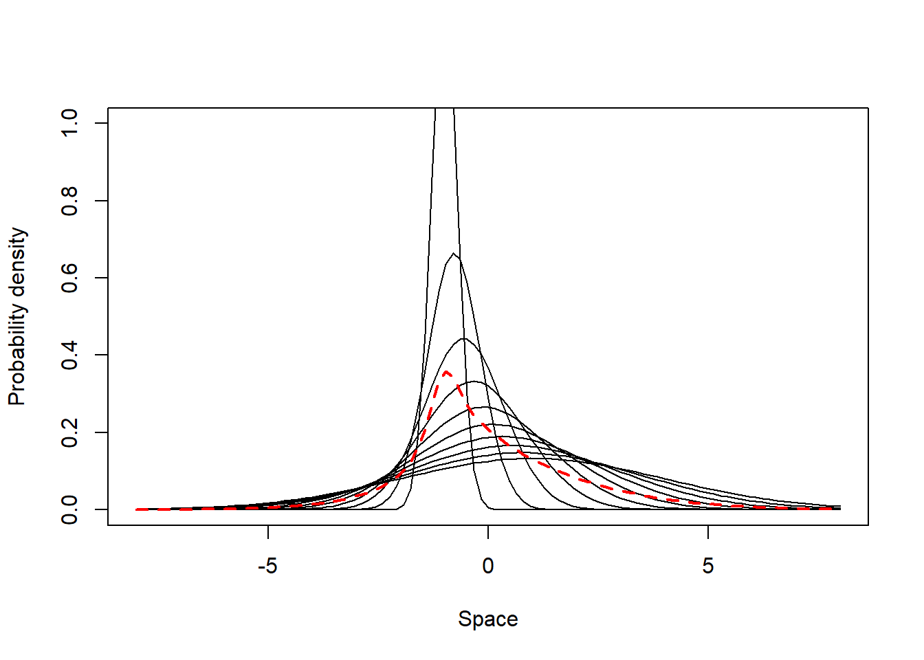
This scenario comprises individuals which are generalist in their most visited places (i.e. have mean UD values close to each other) but do present a gradient of individual variation in their site fidelity - some individuals have UDs with small SD (high site fidelity), while others have UDs with high SD compared to the populational UD standard deviation (low side fidelity). Below we simulate and illustrate such a population.

# Generalist individuals, high interindividual SD variation

# simulate 10 individuals

# individual UD mean
avg.specialist.low <- seq(-1, 1, length.out = 10)
# individual UD SD
# sd.specialist.low <- runif(10, 0, 3)
sd.specialist.low <- seq(0.3, 3, length.out = 10)

# Populational UD
pop.curve <- function(x, mn, sd) {
  f <- 0
  for(i in 1:length(mn)) f <- f + dnorm(x, mean = mn[i], sd = sd[i])
  f/length(mn)
}
# Making sure it integrates to 1
integrate(pop.curve, lower = -Inf, upper = Inf, mn = avg.specialist.low, 
          sd = sd.specialist.low)

## 1 with absolute error < 3.1e-06

# plot
plot(0, 0, type = "n", xlim = c(-8,8), ylim = c(0, 1),
     xlab = "Space", ylab = "Probability density")
for(i in 1:length(avg.specialist.low)) {
  curve(dnorm(x, mean = avg.specialist.low[i], 
              sd = sd.specialist.low[i]), from = -8, to = 8, add = T)
}
curve(pop.curve(x, mn = avg.specialist.low, sd = sd.specialist.low), 
      from = -8, to = 8, lwd = 2, lty = 2, add = T, col = 2)

The populational values of the indexes are relatively low (SpatIS = 0.28, SpatICS = 0.31) and close to those of a typical generalist population (section 2), but still indicate some degree of specialization in the population. This is clearer when observing the individual values: there are individuals that are specialized in some areas (maximum SpatIS = 0.61, max. SpatICS = 0.68), while others are highly generalists (minimum SpatIS = 0.17, min. SpatICS = 0.19). This means this population is composed of a mixture of specialist and generalist individuals, yet is predominantly a generalist population.

# declare SpatIS function 
spatis <- function(i, j) {
  1 - integrate(function(x, md, ss) 
    pmin(dnorm(x, mean = md, sd = ss), 
         pop.curve(x, mn = avg.specialist.low, sd = sd.specialist.low)), 
    lower = -Inf, upper = Inf, md = i, ss = j)$value
}

# declare SpatICS function
spatics <- function(i, j) {
  1 - integrate(function(x, md, ss) 
    pmin(dnorm(x, mean = md, sd = ss), 
         pop.curve(x, mn = avg.specialist.low[avg.specialist.low != md],
                   sd = sd.specialist.low[sd.specialist.low != ss])), 
    lower = -Inf, upper = Inf, md = i, ss = j)$value
}

# calculate SpatIS
# individual values
mapply(spatis, avg.specialist.low, sd.specialist.low)

##  [1] 0.6093993 0.4003052 0.2567049 0.1840565 0.1639828 0.1686378 0.1946920
##  [8] 0.2341482 0.2759718 0.3143370

# populational value
mean(mapply(spatis, avg.specialist.low, sd.specialist.low))

## [1] 0.2802236

# calculate SpatICS
# individual values
mapply(spatics, avg.specialist.low, sd.specialist.low)

##  [1] 0.6771103 0.4447835 0.2852277 0.2045072 0.1822031 0.1873607 0.2163245
##  [8] 0.2601643 0.3066353 0.3492633

# populational value
mean(mapply(spatics, avg.specialist.low, sd.specialist.low))

## [1] 0.311358

Conclusion

This examples demonstrate the application of the indices of individual specialization in the use of space in different ecological contexts, from the typical populations composed of only generalist or specialist populations to the more realistic populations composed of specialist and generalist individuals. These examples show that it is important to look beyond the population SpatIS and SpatICS values to characterize the individual specialization in the use of space within a population. The populational values of these indices may be useful to compare populations, but the distribution of individual SpatIS ad SpatICS values may provide a more in-depth assessment of individual specialization, since it is possible to understand how different individual specialization patterns are spread within the population. Plotting individual and populational UDs may also be very important to understand qualitatively how individual specialization in the use of space occurs within populations.